We promise there was no smoke, no fire, and nobody got hurt. We had to push the limit from the 60 we ran in our article to 72. We thought there was room on the qubits through ad-hoc observation for 20% more stocks when we published our last article here.
Why try 72? We know this will push our classical solvers a little harder, but should still work quickly and accurately. On August 21, 2020, we attempted to run 72 stocks through our classical and quantum methods. It failed to embed on the D-Wave quantum annealer. Classically, we met with mixed success. In short, we must make progress to successfully execute 72 assets.
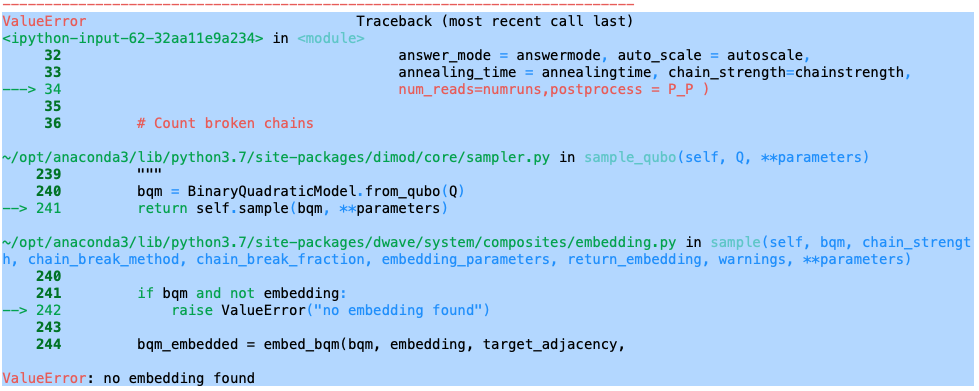
The error message we received was “no embedding found.”
Let’s walk through the full lifecycle of the analysis, from start to finish.
Alex Khan picked 72 story stocks and active stocks that have a large following, high market capitalization, and many of them have news and speculation interest. We found that three of the stocks had negative BETA (they go down when the market goes up), so we replaced them with positive BETA stocks. The 72 final stocks have all been continuously trading for 253 days.
The hilbert space, or number of stock portfolios to evaluate, is 4.722 * 10²¹. This is 4,096 times larger than the 60 stock analysis. So, 72 stocks is a significant increase in the complexity of the problem we are trying to solve.
We download the data, we load the counters, we calculate the market indices (risk free rate we use is 1%, but the calculated value is 0.90%, and market return is 18.23%). We check the BETA values and see a wide spread (0.298, 1.81). We calculate the ‘all-in’ 72 asset portfolio values. The expected return is 20.10%, and the expected standard deviation is 2.32%, based on the Capital Asset Pricing Model. This assumes the variance of the portfolio carries forward from the past 12 months, and the expected return is calculated using the weighted average of the BETA terms against the market index.
The ‘plumbing’ or mechanical aspects of our algorithms execute well for 72 assets, as they did for 60 assets.
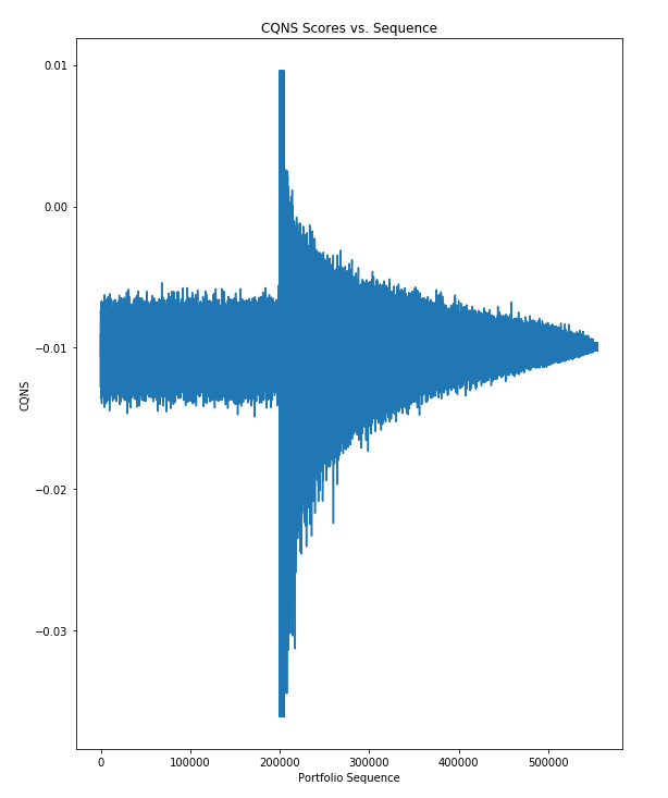
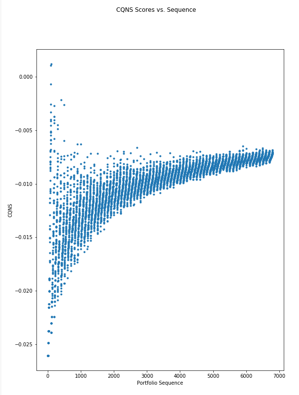
When we run the Monte Carlo analysis, we see the smallest portfolio sizes (1,4) have the best outcomes. In the chart below, we see the first truly random Monte Carlo analysis (the first 200,000 samples) give us a broad range around -0.01. Then we hit the fat-tailed Monte Carlo analysis which is sequential based on portfolio size. It shows the best and worst portfolios (lowest and highest scores), and the largest spread, at the smallest portfolios. In other words, the CQNS score predicts that investors will have best and worst options if they hold just a few stocks.
T0he best answer found is one asset, with a CQNS value of -0.036064, followed by a 2-asset answer, then a set of (2,4) asset answers. We will stay with this ‘ideal’ solution for this run, but likely will adjust our model to select 2+ asset solutions. In our mind, one asset is not a portfolio.
The range of the CQNS scores shrinks as the portfolios get larger. In other words, if you are going to hold many stocks (say 36+ out of 60 stocks, you will average out to the middle of the random range.
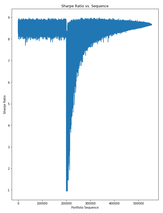
It is important to note the Sharpe Ratio has a different shape, and method of finding attractive, efficient portfolios. As seen below, the Sharpe Ratio ranges from (8,9) for the set of random samples. Then, for the smallest portfolio the Sharpe Ratio does not find attractive portfolios. If we eyeball the chart below, we see the best portfolios come in between 200k and 300k, which is around portfolio sizes (10,30). There are no best answers in small portfolios.
We then write out the counters and run our genetic algorithm seeded with random samples. It completes in 52 seconds, and does find the same ‘ideal’ solution.
We run our simulated annealer from D-Wave. This solver is set so it finds portfolios with 2 or more assets. It finds 97 valid portfolios in 8 seconds, and many of them contain the ‘ideal’ stock chosen by the Monte Carlo analysis. Portfolio sizes include (2,3,4,5,6,7,8,9,10, 15). This looks like a reasonable run selecting a small number of attractive portfolios to further analyze.
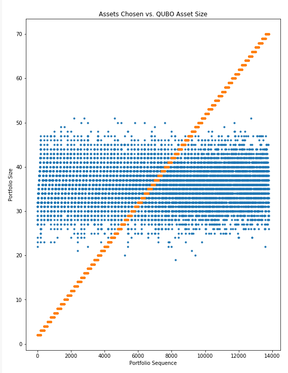
In the chart below we can see the CQNS scores (adjusted by the D-Wave simulated annealer and penalized by our QUBO) against the portfolio sizes. The higher the sequence, the larger the portfolio (2,69).
We then run the bespoke or custom simulated annealer from Chicago Quantum. This one selected a 3-asset solution with a similar score to the Monte Carlo 1-asset solution (CQNS score of -0.033213), and included the ‘ideal’ stock in the solution. It ran in 44 seconds. It found the same answer with a faster setting, but we had deepened the annealing range (let it run longer) to see if it changed its result.
We ran the D-Wave Tabu sampler for portfolio sizes (2,70), and received valid portfolios (24,50), with a mix of positive and negative scores right around zero. This analysis took 345 seconds, and did not yield useful portfolios when scored by the CQNS.
What we see below is that the Tabu sampler finds portfolios in the range of ~ 20 to 52 despite the penalty on the score, and the portfolio sizes desired by the QUBO. We see this in the blue dots being fairly consistent (the answers) despite the linear progression of the portfolio sizes desired (orange dots).
We ran the D-Wave Hybrid Solver. We asked for valid portfolios at three sizes (3,36,60). Unfortunately, it could not match the solutions to the sizes desired. It returned a 2-asset portfolio when asked for 3, 20 vs. 36, and 32 vs. 60). So, we cannot use these answers.
Now we close the files and get ready to run the D-Wave quantum annealer. We set up the job to run 200 samples, a chain strength of 1, and a relatively long annealing time of 100 microseconds. It did not complete, but return an error that it did not successfully embed the problem on the D-Wave quantum annealer. We validated this with a look through documentation and community / FAQ / trouble shooting postings.
As this procedure did not run, we cannot run the D-Wave Inspector and see where the problem failed. We must reformulate the problem to successfully embed and run on the D-Wave before we can see the qubit values, chains and open spaces left on the QPU.
This is part of our work for this week…to figure out how to fit 72 stocks on the QPU.
Update 1: There seems to be a theoretical maximum limit for a complete graph where all stocks (vertices) connect to all stocks (vertices) of 65. This assumes 100% access to the 2,048 qubits. 2MNL = 2*16*16*4 = 2,048. https://docs.dwavesys.com/docs/latest/c_handbook_5.html
We see the cap of 65 stocks at one time on the D-Wave quantum annealer with the Chimera topology. We are still working to scale up our classical methods, and will wait until we have access to the Pegasus architecture to continue scaling our quantum annealing runs.
This does mean that our quantum offering to investors and investment managers will scale up to 64 assets.
August 26, 2020 update:
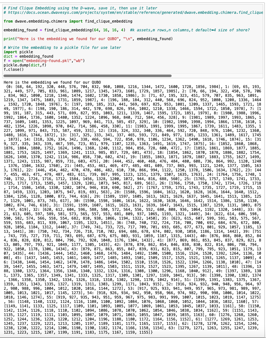
So, we found out that the Chimera graph (16,16,4) can theoretically support embedding of a full 65 element graph where all the vertices are connected (e.g., all stocks are connected to each other). This is called a clique. Thankfully, we can run a D-Wave function named: find_clique_embedding and find an embedding for our problem. We only get this to work up to N=64 stocks, so that becomes our limit moving forward.
The output looks like this. We write it to a pickle file for later use with a D-Wave sampler aptly named: FixedEmbeddingComposite.
Now we go back to hardening our analysis and ensuring both our quantum and classical code works great. We are tuning our CQNS formulation, and will be improving the user interface.
For more information, drop us a line at [email protected]
Re-published with permission. Source: M. Jeffrey Cohen, Quantum Stock Portfolios…
Content may have been edited for style and clarity.